What is digital audio? A complete guide for artists
Independent artists around the world use digital audio to make music in their home studios everyday.
Thanks to digital audio, home recording equipment is far more affordable than it was in the days of analog. Rewinding 30 to 40 years and recording music was a drastically different process.
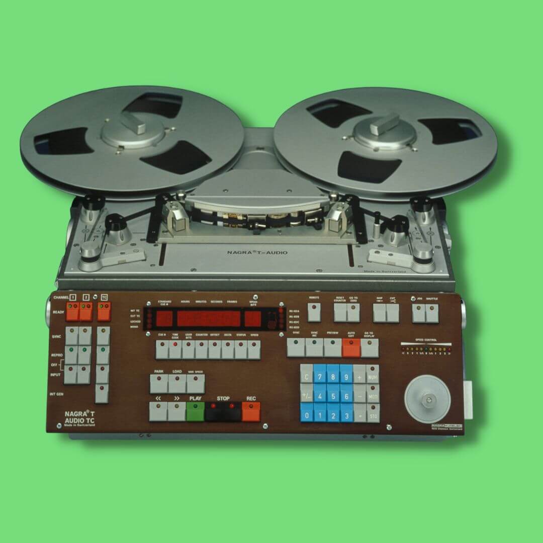
Back in the 70s, you’d have needed some chunky equipment like a reel-to-reel tape deck to record anything professionally at all. Now you just need a semi-decent computer and an audio interface!
To understand why digital audio has made such a positive impact on the music industry and created an ever-growing web of independent artists, we’re going to explore the following topics:
- What is the difference between analog and digital audio?
- Digital audio resolution (PCM)
- Digital distortions
- Making music with digital audio
- Exporting your digital music production
What is the difference between analog and digital audio?
Digital audio technology converts sound waves into digital/binary data that a computer can read.
Meanwhile, analog technology like a microphone converts sound waves into electrical signals that rely on circuit technology.
To record at home today, you’ll need an audio interface and a laptop. However, if you were recording at home in the 70s then you’d have needed a reel-to-reel tape deck or a cassette.
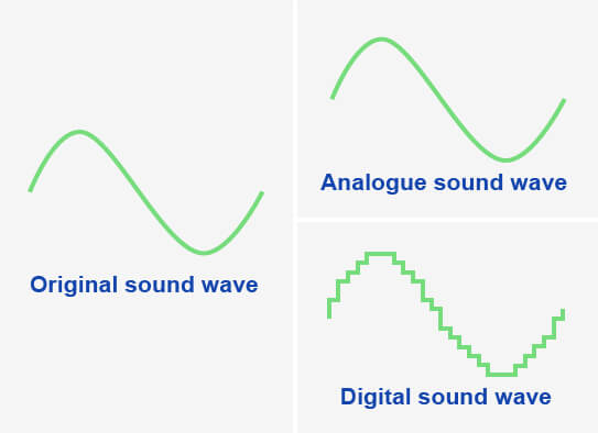
‘Analog’ recording imprints a waveform onto tape via charges or onto vinyl via grooves.
Then, we can play the recording back in speakers via an electromechanical transducer.
For example, a tape deck reproduces an electrical signal from the tape for the speakers to play after amplification.
In contrast, a vinyl stylus (the needle) generates an electrical signal as it scratches the vinyl grooves and transports the signal via wire to an amplifier.
With that said, vinyl is only a means of playback while a tape deck is a means of recording and playback.
It’s often said that digital recording can’t reproduce a soundwave as accurately as analog.
Both analog and digital recording tech can reproduce the original audio perfectly.
This isn’t true for reasons we will explore together throughout this post.
Analog to digital conversion (ADC)
The two processes of recording with analog and digital technology are incredibly different.
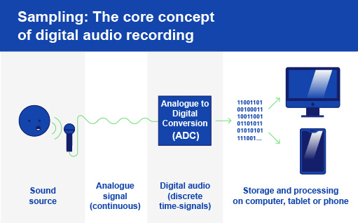
While analog recording equipment imprints soundwaves as electrical charges on magnetic tape, at the core of digital audio is sampling.
For example, a digital device like an audio interface will take snapshot samples of an input signal at specific intervals.
Altogether, this process of sampling audio and converting it to digital is called Analog to Digital Conversion (ADC).
A fitting name, don’t you think?
So rather than imprinting a soundwave onto analog tape or vinyl, ADC samples a microphone or instrument’s electrical signal at specific points in time to reconstruct it in the digital realm.
And once the A2D conversion is finished, you can store or send this digital audio file to a digital device such as a computer, an iPad, or a smartphone.
Moreover, on computers, we can process digital audio files in a DAW in what seems like an unlimited amount of ways. And this is called digital signal processing (DSP).
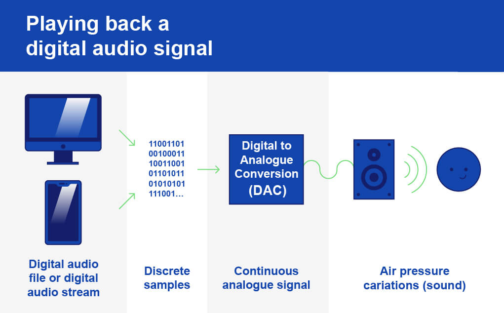
To illustrate this concept, the diagram below shows how DSP is used in an MP3 audio player during the recording phase.
After ADC, DSP captures the digitized signal and processes it. Once we’re done, we can send the signal back out into the real world, so to speak.
However, when you listen back to the digital audio through headphones or speakers another process must occur before the audio reaches your ear.
This process is the reverse of Analog to Digital – it’s Digital to Analog Conversion (DAC). Through the DAC process, digital equipment like an audio interface reconstructs the original analog (electrical) signal from the digital signal and powers the speaker cones.
Finally, both the ADC and DAC processes utilize filters that smoothen the final audio throughout recording and playback.
A low pass antialiasing filter ensures there are no frequencies too high in the signal. In other words, an antialiasing filter ensures all frequencies in the signal are sampled correctly in the ADC.
Don’t worry if that last bit is a bit confusing. We’re coming back to aliasing later on with lots more detail!
Finally, a smoothing filter interpolates the waveform between the samples during the digital to analog conversion too. In other words, the interpolating filter ensures the segments between the sample intervals represent the original signal.
Digital audio resolution
If you’ve been shopping for audio interfaces before then I know you’ve seen the phrases “sample rate” and “bit depth”.
Well, those are concepts that determine the quality of the digital reconstruction of an analog signal, or audio resolution for short.
Digital image resolution and color information depend on pixel amount and bit depth. Likewise, the resolution of a digital audio signal depends on sample rate and bit depth.
In digital audio, both sample rate & bit depth work to create a total bandwidth that defines the quality of our digital audio signal.
Therefore it’s the bandwidth that defines how accurate our digital signal is compared to our original signal.
More bandwidth = more accurate reproduction
In contrast, the accuracy of analog gear depends on the sensitivity of the recording equipment you’re using!
Sample rate
The number of sample measurements taken per second, and therefore also the speed at which they’re taken, is the sample rate.
To reproduce any signal near-accurately, thousands of samples must be taken from an audio signal per second.
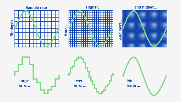
In the image below, you can see that taking more samples per second gives us a smoother waveform.
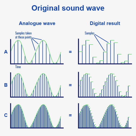
The digital result in example A is blocky and it doesn’t capture the smoothness of the original audio signal.
But the digital result in example 2 takes more samples of the audio signal and gives a closer representation of the audio signal.
In the final example, we’ve taken enough samples to reconstruct the audio signal accurately.
So the sample rate of a digital signal describes the number of samples taken and the speed at which they were taken.
As you’ll notice when shopping for an interface, the unit of measurement for sample rate is kilohertz (kHz).
This means that the common sample rate of 44.1 kHz translates to 44,100 samples taken per second.
A list and a brief history of sample rates
To understand why 44.1 Khz is the most common sample rate, we have to back in time.
When digital audio was first entering the scene, file size and storage capacity was a big concern. After all, computers were not what they are now – storage was quoted in megabytes, not gigabytes or terabytes.
That’s one reason the CD standard of 44.1 kHz was and is a decent halfway line between audio quality and mitigating storage issues.
But the main reason it became the standard CD format is because a sample rate of 44.1kHz is enough to reproduce the frequencies humans can hear – for reasons we will shortly explore.
Below is a list of the common sample rates:
- 44.1 kHz 44,100 samples per second
- 48 kHz – 48,000 samples per second
- 88.2 kHz – 88,200 samples per second
- 96 kHz – 96,000 samples per second
- 192 kHz – 192,000 samples per second
While shopping for any recording gear, it’s essential to note that you can’t record in any resolution that exceeds that of your interface.
To illustrate, you can’t record at 96kHz if your interface has a limited sample rate of 44.1kHz. Make sure you look at the tech specs!
How the sample rate affects your digital signal
If you’re looking to record a stereo signal, recording at 44.1 kHz will not do unless you record each channel individually (as is the common practice).
Recording in stereo gives you double the signal to capture. Therefore you’ll need to double the sample rate at which you’re recording to 88.2 kHz!
In other words, recording a 1-second long stereo file requires you to take 88,200 samples.
A soundwave is made up of cycles. Furthermore, each cycle has one positive and one negative amplitude value – the measure of its signal strength.
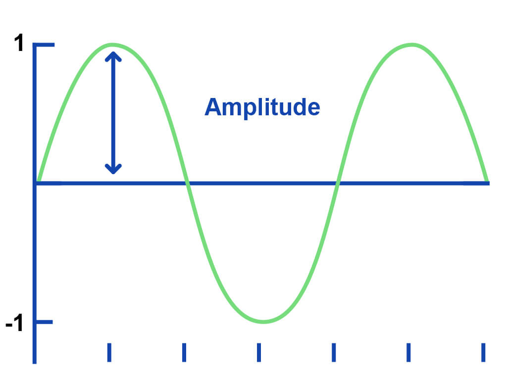
To find its wavelength – the length of an individual cycle – we need to measure both the positive and negative amplitudes of said cycle.
As a result, we must sample every cycle’s positive and negative amplitudes in the ADC process to accurately measure and reconstruct the amplitude of the original signal.
And sampling every cycle twice is the minimum amount required to avoid aliasing.
Aliasing: why do we take at least two samples per cycle?
But the process of sampling can go wrong.
Taking too few samples per cycle leads to the DSP unit interpreting the soundwave incorrectly and creating an unwanted ‘alias‘ of the original.
An alias is an unwanted false representation of a soundwave. To demonstrate, let’s take a look at these examples:
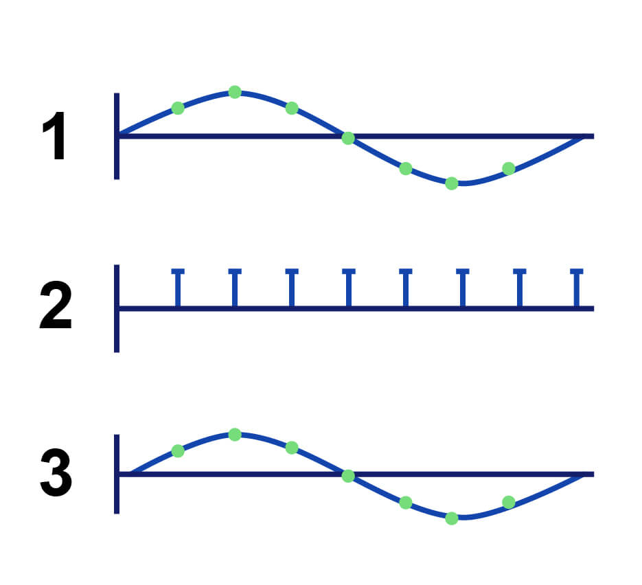
Taking the correct amount of samples leads to an accurate reconstruction of the soundwave. 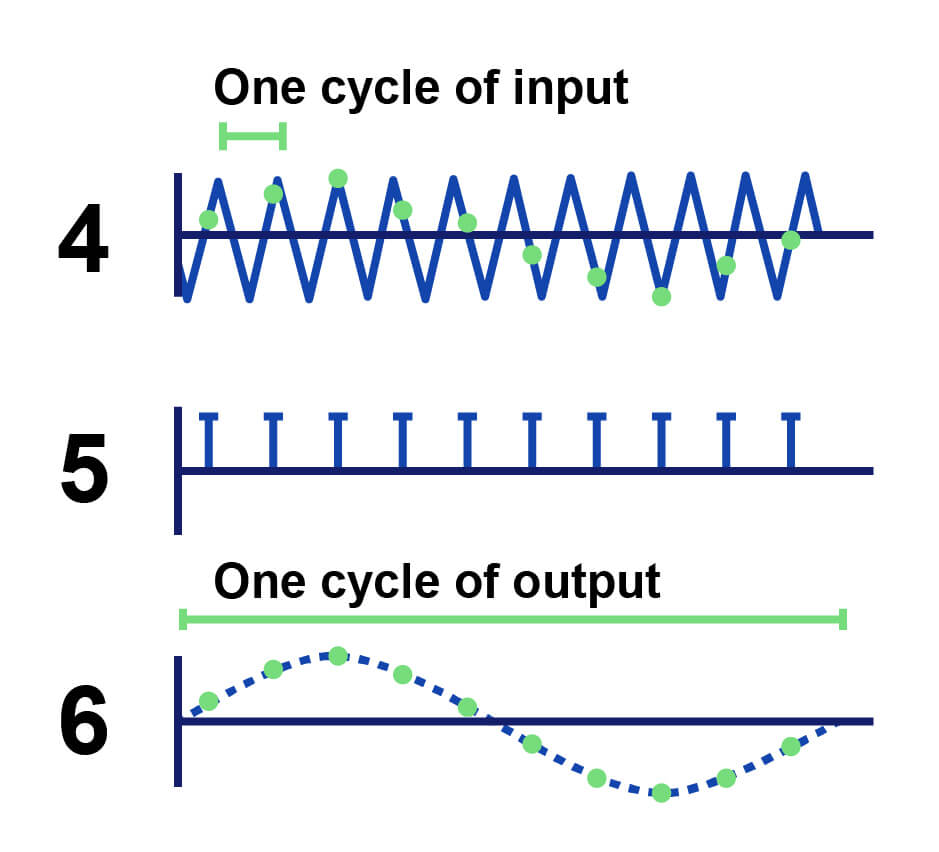
Taking too few samples of a soundwave leads to reconstruction with too low a frequency.
In the first image, the reconstructed soundwave (3) resembles the original soundwave (1) perfectly. That’s because enough samples were taken (2) to capture the frequency of the soundwave.
But in the second image, we haven’t increased how many samples we want to take (5) despite rapidly increasing the frequency of the audio (4).
As a result, our reconstructed waveform (6) resembles that of the first example with a much lower frequency.
Nyquist-Shannon Theorem: the method behind the madness
With these above examples in mind, you can see why we need to take at least two samples per wave cycle.
Taking two per cycle gives us a digital waveform with the frequency information of the original wave intact.
So taking less than two cycles per second leads to a digitized signal with too low a frequency than our original signal.
Therefore we can conquer that we need a sample rate of at least double the highest frequency of our signal. And this is what we call the Nyquist-Shannon theorem.
Using the most common rate as an example, the highest frequency we can record at a sample rate of 44.1 kHz is 22.05 kHz. This is perfect for us humans as our ears can only hear frequencies between 20 Hz – 20 kHz.
Though we could use a higher sample rate, we do still have the issue of a bigger file size. As we discussed earlier, 44.1 kHz became the standard sample rate due to (lack of) storage space and audio quality.
However, with the Nyquist theory, it’s clear to see that 44.1 kHz is a sample rate high enough to capture all frequencies that humans can hear.
Using a higher sampling rate does have its uses though. Sampling frequencies above the threshold of human hearing allows you to capture the nuances in the upper-frequency range which can add value to the listening experience of a track.
Unfortunately, fans will only be able to play your track at 44.1 kHz on streaming services like Spotify anyway.
No matter how high a sample rate you use while recording, CD quality audio is the standard for streaming services.
Bit depth
After sampling the audio, your computer needs to store your recording. And computers store information in binary 1s and 0s, otherwise known as bits.
The number of available bits determines the number of amplitude values that a digital system can store. By way of illustration, more bits allow for more storage space.
Soundwaves are continuous waves, meaning they have a countless number of possible amplitude values.
So to measure sound waves accurately we need to establish their amplitude values as a set of binary values.
Going back to our digital image example, if you had a 4K image but a low bit depth then the colour of the image wouldn’t be very exotic despite the potential details available with 4000 pixels!
Likewise, recording a 1-second audio signal with a sample rate of 96kHz but an 8-bit depth really limits how your gear can map those 96,000 samples to digital bits. What you’d get is something like this:
You can see how sample rate and bit depth work together to reconstruct one wave cycle in the image above.
As a result, the result of more available bits is a wave cycle that’s much more accurate due to the correct mapping of amplitude values.
The popular bit depths are 16-bit, 24-bit, and 32-bit, but bear in mind that these phrases are just binary terms that represent the number of possible amplitude values available.
- 16-bit = 65,536 amplitude values
- 24-bit: = 16,777,216 amplitude values
- 32-bit = 4,294,967,296 amplitude values
While 24-bit depth provides more bits than 16-bit depth, there is almost no point in recording with any higher than 16-bit due to the standards of streaming stores.
As with the 44.1 kHz sample rate issue, stores require tracks to be in 16-bit too. So streaming stores quite literally ask for CD quality audio (44.1 kHz sample rate with 16-bit depth).
But a higher bit depth gives you:
- Greater dynamic range
- A greater signal-to-noise ratio (SNR)
- More headroom before clipping occurs while recording
Take note, though, that a higher sample rate and bit depth will also give you a bigger audio file too.
How to calculate the file size of your digital recording
Using the sample rate, bit depth, and the number of channels in our project, we can calculate what its file size will be when we export it as an audio file.
The following formula will give you the bit rate of your audio file, measured in megabits per second (Mbps).
Sample rate x bit depth x number of channels = bit rate (Mpbs)
The bit rate of your audio file determines how much processing your computer must undertake to play your audio file.
So let’s say we record one guitar riff with a sample rate of 44.1 kHz and 24-bit depth.
44,100 x 24 x 1 = 1,058,400 / 1.1 megabits per second (Mbps)
Then, after calculating the bit rate of your recording, multiply it by the number of seconds of your recording. Let’s say we recorded for 20 seconds.
1.1 x 20 = 22 / 22MB
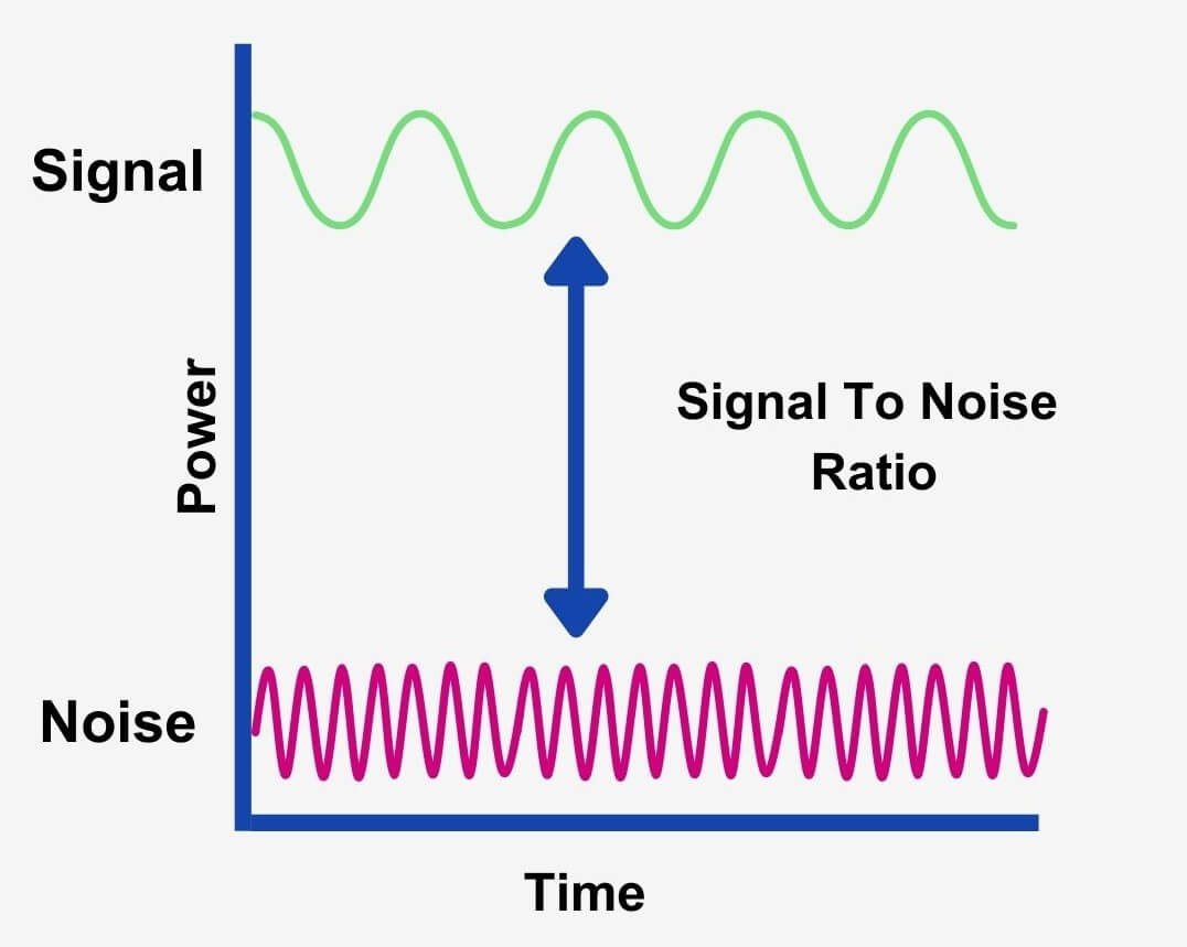
What is the Signal-to-Noise Ratio (SNR)?
SNR refers to the difference in level between the maximum signal strength your gear can output relative to its inherent electrical noise, measured in dB.
All electrical equipment produces noise. But a higher bit depth in recording gear allows for a louder recording before the noise becomes apparent.
The noise of equipment can be a negative number, a positive one, or even zero. In fact, an SNR over 0 dB tells us that the signal level is greater than the noise level. Therefore we can see that a higher ratio means better signal quality!
So if your interface has a noise floor of 100dB, this means that you can record at a level up to 100dB before noise infiltrates your signal. In other words, a higher number means a better signal-to-noise ratio.
This is why we wouldn’t push our input gain as hard as we can while recording. Doing so may only make the noise floor of our device more apparent.
In summary, higher bit depths do give us a lower noise floor.
What is dynamic range?
The dynamic range of a signal is the difference between its loudest and softest parts of a signal, measured in decibels (dB).
And if a digital system like an audio interface has 100 dB of dynamic range, this means it can accurately register signal strengths between -100 dBFS to 0 dBFS (decibels at Full Scale).
Dynamic range is important in music due to how our hearing works. To perceive something as loud, we need to perceive something as quiet – like a frame of reference.
So a greater dynamic range in recording gear allows for a bigger contrast between loud and quiet sounds in your recording.
And we can calculate the maximum dynamic range of a digital recording like this:
Maximum dynamic range in decibels = number of bits x 6
8 x 6 = 48dB of dynamic range – less than the dynamic range of analog tape recorders.
16 x 6 = 96dB of dynamic range – ample room for recording. But for hi-res audio, we need more.
24 x 6 = 144 dB of dynamic range
From this brief maths session, we can see that a higher bit depth allows us to record a louder signal with more clarity.
With these two rather confusing concepts in mind, we only really need a bit depth with an SNR high enough to accommodate the dynamic range between the softest and loudest signal strength we want to record accurately.
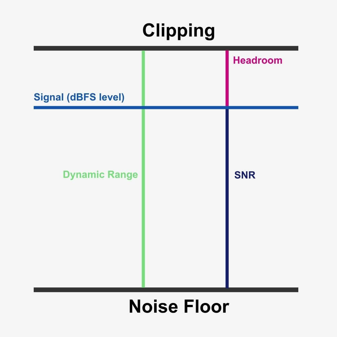
Additional headroom
Finally, headroom is the difference between your loudest peak level and the 0dBFS ceiling.
For illustration, driving a 4-meter high bus through a 5-meter high tunnel gives you 1-meter of headroom.
With 144 dB of dynamic range available with a bit depth of 24-bit, we can avoid clipping with ease while practically eliminating our noise floor too!
Digital distortions
You may be thinking that using a higher bit depth to achieve a higher dynamic range means we can record as loud as we can. As fun as this would be, recording as loud as you can is not necessary. In fact, it’s counterproductive.
If you do then you’re likely to ‘clip’ your signal in your DAW.
But before we dive into that, let’s talk about this ‘dBFS’ metric we’ve been talking about.
What is dBFS?
Decibels relative to full scale (dBFS or dB FS) is a unit of measurement in digital systems. More specifically, we use dBFS to measure amplitude levels like those in pulse-code modulation (PCM).
All digital audio gear, whether an audio interface or a DAW, uses dBFS to measure the amplitude of signals.
0 dBFS is the maximum level a digital signal can reach before clipping interferes with your signal.
Furthermore, a signal half of the maximum level is −6 dBFS (6 dB below full scale).
This is so because 6dBFS doubles the volume of your signal.
Peak measurements smaller than the maximum are always negative levels.
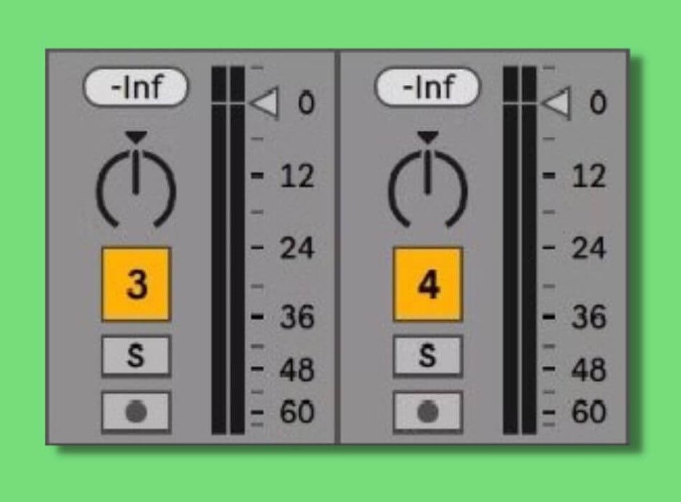
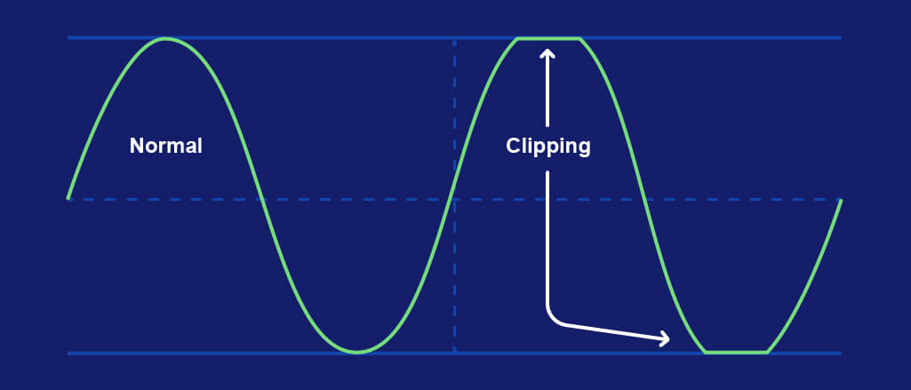
And when your signal exceeds 0dBFS it will clip – a form of digital distortion.
Clipping
Before I confuse you, a higher bit depth does allow for more headroom before clipping the output on your recording gear. However, it does not allow for more headroom in your DAW.
Recording at a higher bit depth only allows for more headroom on your recording device.
By recording at a level higher than 0 dBFS you’ll hear a noise sounding like horrible static in your signal. In actual fact, clipping squares off the soundwave – where the ceiling and floor flatten the positive and negative amplitudes.
If you are clipping your signal while recording then that static sound will be in your recording. And once it’s recorded, you can’t get it out.
No matter how much dynamic range your audio interface gives you, your dBFS ceiling is the final boss – and it’s unbeatable. Therefore we must use gain staging while recording and mixing if we want to keep our signal clean and preserve its dynamics.
Keep those faders down!
Digital clipping vs analog distortion
Analog distortion, on the other hand, occurs when your input signal is pushed louder than the peak voltage of a particular piece of analog gear can handle.
Digital clipping sounds the same no matter what plugin, gear, or sound has overdriven the signal. But analog distortion will sound different on different pieces of analog hardware.
In short, this means that digital clipping doesn’t inherit any unique characteristics of a particular piece of gear or software. But analog distortion can change based on the unique circuitry of the hardware that the signal is traveling through!
Quantisation error/noise
Due to their fluid shape soundwaves won’t always line up with an available bit. Especially in bit depth below 24-bit, one amplitude value of the soundwave is going to sit between two bits.
As a result, the ADC converter in your interface will round it off to the nearest value – known as quantizing.
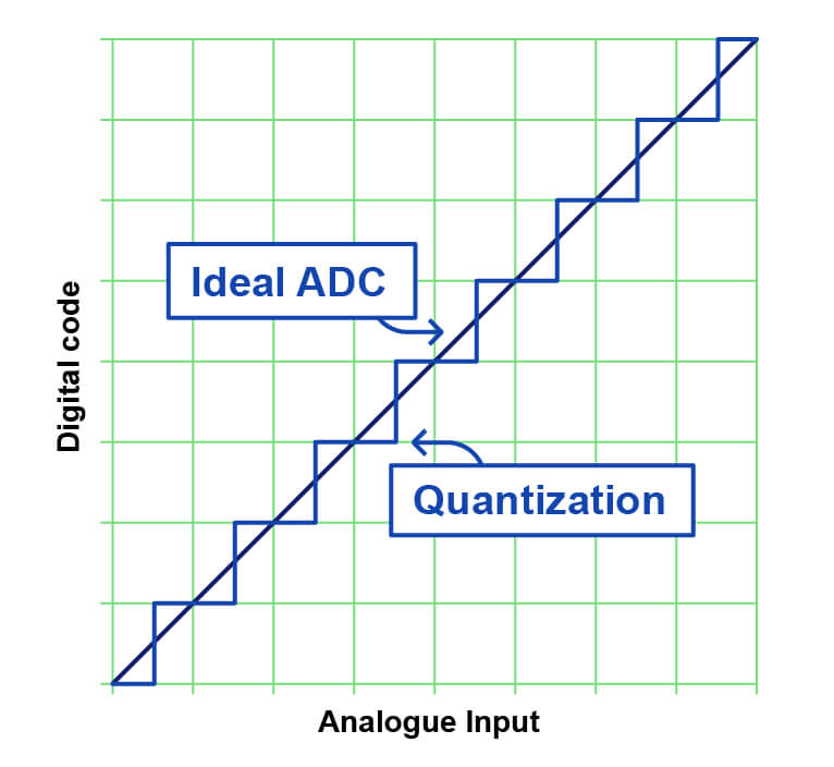
And rounding a soundwave to a bit that doesn’t accurately represent its amplitude leads to quantization distortion.
This is because of the limited number of digital bits available.
Information gets deleted and ‘re-quantized’ when reducing the bit depth of a file, resulting in a grainy static sound – quantization noise.
This is mainly a problem when decreasing the bit rate of a pre-recorded file.
So when a 24-bit file is reduced to CD – 16-bit/44.1kHz – that’s when quantization distortion becomes a problem.
Therefore, quantization noise is the difference between the analog signal and the closest available digital value at each sampling instance.
Quantization noise sounds just like white noise because it is just that. However, it sounds more like distortion when you lower the bit depth severely.
This process of re-quantization creates certain patterns in the noise – correlated noise. Correlated noise is particular resonances in definitive parts of the signal and at particular frequencies too.
These resonances mean our noise floor is higher at these timestamps than elsewhere in our track. In other words, the noise is swallowing amplitude values that our digital signal cannot get access to.
But correlated noise isn’t the kind of gatekeeper we want to come across. Thankfully, there is a way of reducing correlated noise so it’s unnoticeable to listeners upon playback.
What is audio dithering?
In our above example of bit depth reduction from 24-bit to 16-bit, the dithering process adds random noise to the lowest 8-bits of the signal before the reduction. Though this fail-safe is in place, avoid alternating between bit depths!
Increasing the bit depth to 24-bit after you have reduced it will only add more distortion to your signal and you will lose quality.
As we mentioned earlier, severely reducing the bit depth of an audio file will add severe quantization noise. And applying dither to that signal would look something like this:
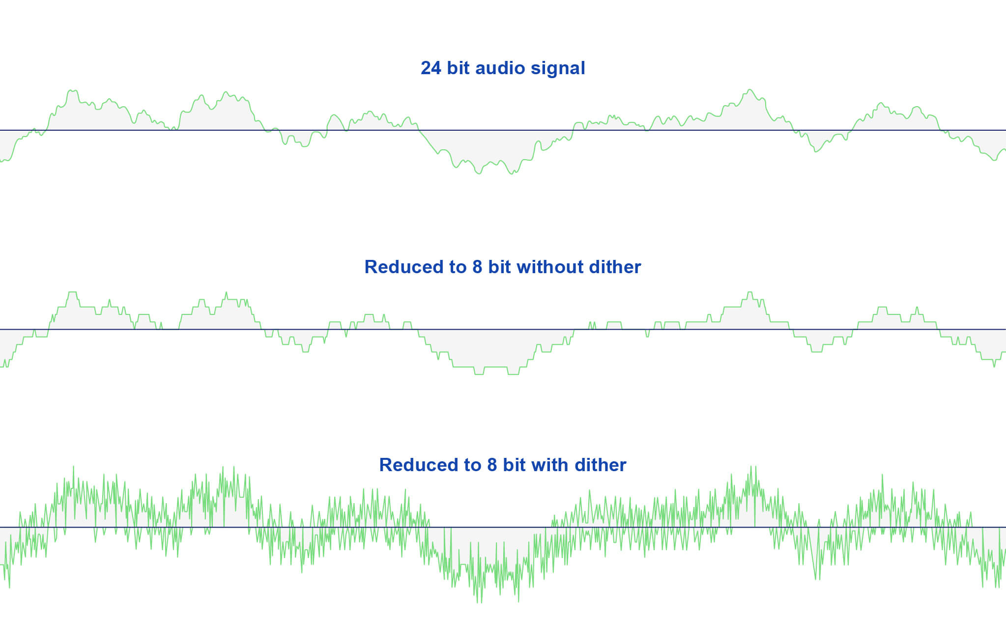
In practice, dithering hides quantization error by randomizing how the final digital bit gets rounded and masks correlated noise with uncorrelated noise (randomized noise).
As a result, the dithering process frees up amplitude values and decreases the noise floor.
We should say that DAWs automatically utilize algorithms to take care of dithering. You don’t need to worry about it so much, but it’s handy to know about.
Making music with digital audio
All of that technical information can be a little jarring, right?
Well, hold on to your hat. Now it’s time to discuss the equipment and software that makes music-making so accessible for independent artists and home studios: DAWs, audio interfaces, MIDI keyboards, virtual instruments, and plugins.
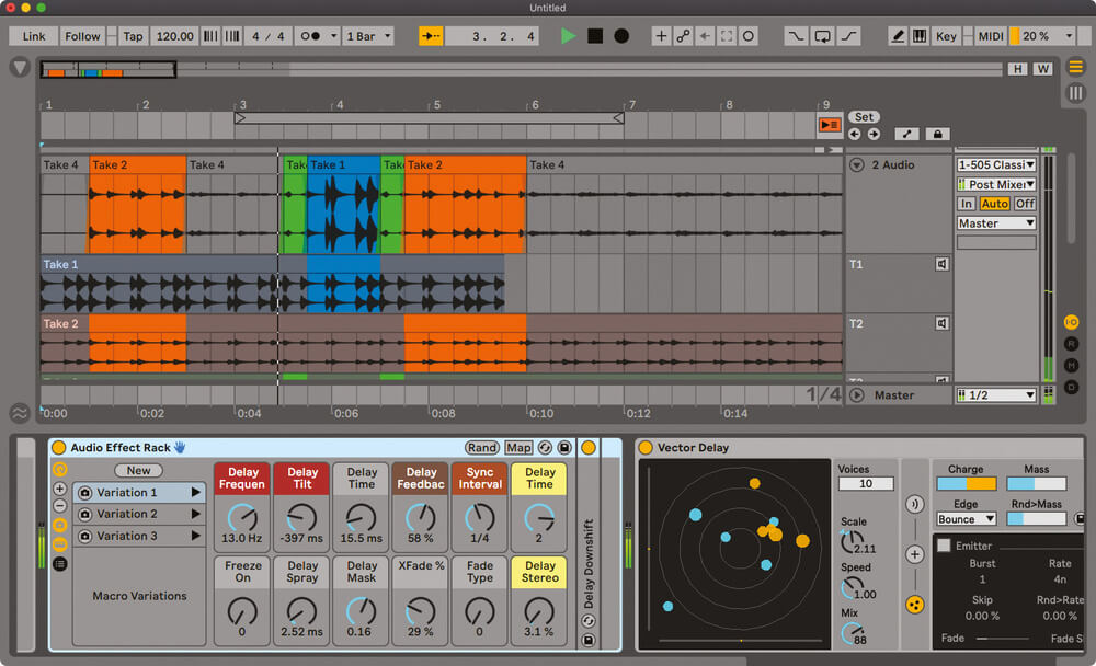
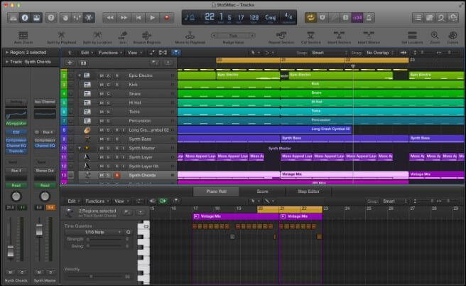
What is a DAW?
A Digital Audio Workstation (DAW) is software that allows us to record and edit our audio, apply a huge range of effects to instruments or groups of instruments, and mix all of our instruments so they work together in a song.
Each DAW has its own quirks and unique features, but the principle is the same for all. We use them for recording and editing audio & MIDI, mixing, and mastering.
After the ADC process, your computer receives your digital audio and feeds it into your DAW. Once inside, you’ll find numerous DAW controls and tools that allow you to manipulate your recording too.
Moreover, every DAW, whether Reaper, Pro Tools, Ableton, Cubase, etc, has its own project file formats for storing projects too.
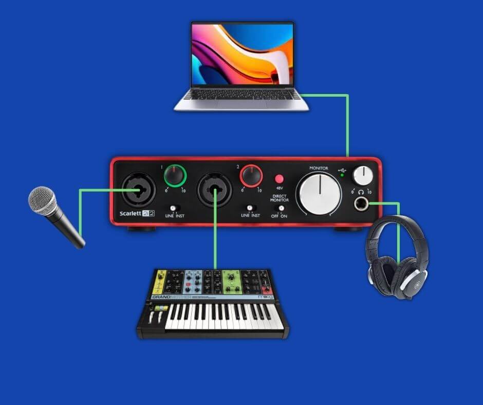
Audio interfaces: ADC converters for home studios
After touching on them briefly, it’s a good idea to talk more about audio interfaces.
An audio interface is the most common example of a digital recording device. While recording with an audio interface, the ADC converter utilizes every principle we have discussed – sample rate, bit depth, dynamic range, etc. – and converts your performance into a digital signal.
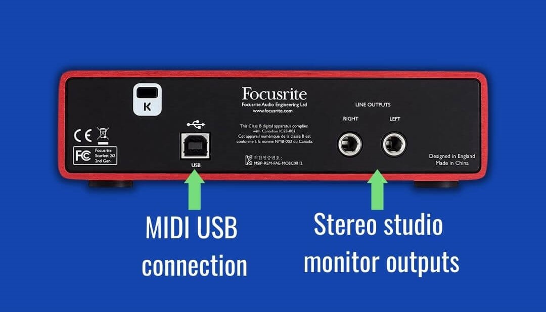
Interfaces connect to computers via USB Type B cable, so no auxiliary cable is required for computer connectivity. Furthermore, interfaces leverage XLR and 1/4″ jack inputs for connecting microphones and instruments.
To get the most out of your interface, it’s important to investigate the tech specs when you’re shopping for an interface. The audio/recording resolution that different interfaces offer. Below is a list of the important specifications to look out for:
- Sample rate
- Bit depth
- Dynamic range
- THD+N – all output leaving your interface that isn’t your signal (electrical noise)
- Frequency response
Most interfaces have a frequency response between 20Hz and 20kHz. The frequency response of an interface determines how an interface captures and processes the frequencies of a given signal.
On a product page, you’ll notice that the frequency response will display like:
20Hz – 20KHz, ± 0.01 (dB).
The value that follows the ± represents volume cuts and/or boosts at specific frequencies. Therefore – in this brief example – the interface will only apply cuts or boosts of 0.01 dB.
Now that we understand how computers receive signals, and how audio interfaces and DAWs make home music production possible, let’s talk about another digital production tool. It’s time to talk about MIDI.
Recording with MIDI
MIDI stands for Musical Instrument Digital Instrument, and it’s become a staple of modern music production.
A MIDI controller provides you with a physical interface for recording virtual notes in a DAW.
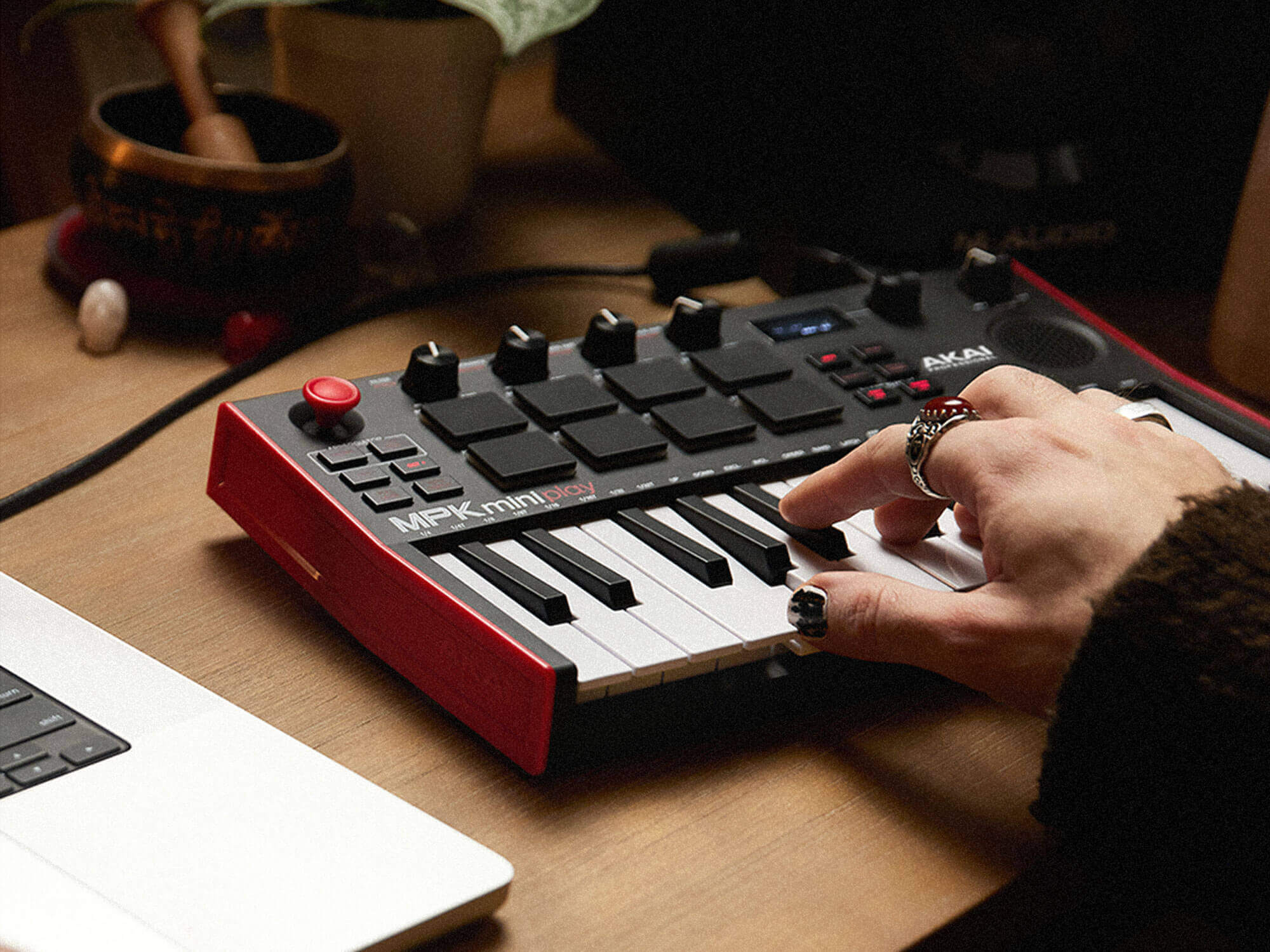
You can also use them to control virtual instruments, plugins, and your DAW itself – not to mention other MIDI controllers!
A MIDI recording only captures information that describes how you use the MIDI keyboard, which in turn manipulates software instruments, your DAW, etc.
This requires a simpler setup than recording audio – all you need is a
- MIDI keyboard
- USB Type-B cable
- A DAW
- A computer
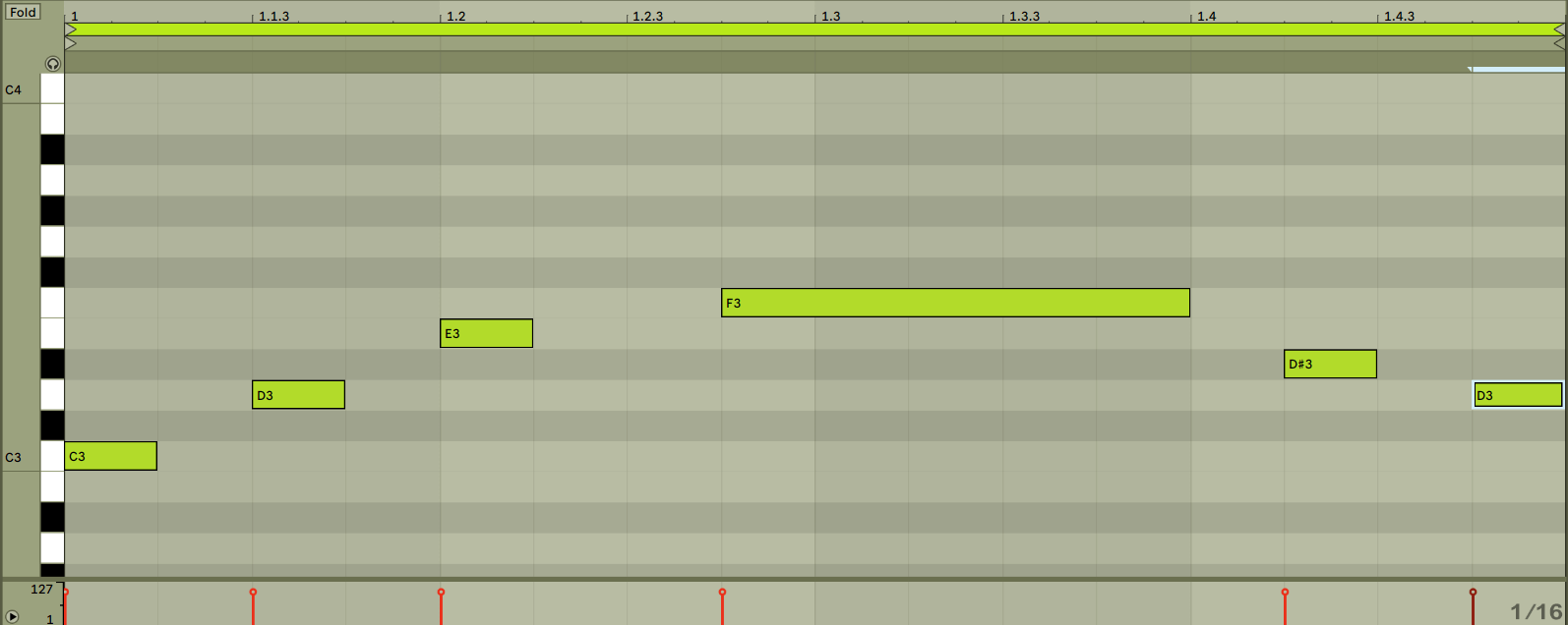
As we play, our DAW draws little blocks in its piano roll that virtually represents the notes we press on our hardware.
Don’t worry, I’ll come back with more detail on these little blocks.
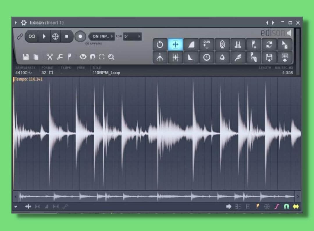
In contrast, converting an audio signal into a digital one gives us a visual waveform of our recording.
Via a USB Type B cable, sometimes known as MIDI over USB cable, we can connect MIDI keyboards (and audio interfaces) straight to our computer and software thusly.
With that said, some audio interfaces even provide a USB input now too, so we can connect MIDI straight to our interface instead.
On the other hand, we can use 5-Din MIDI cables to connect different MIDI controllers to one another in the same signal chain if our MIDI controller has the correct port.
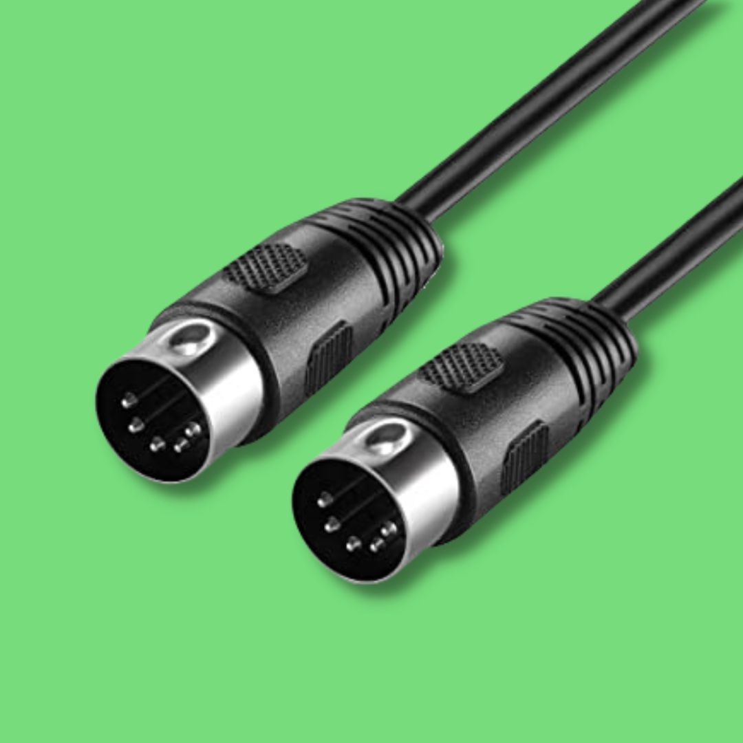
5 DIN MIDI cable for connecting MIDI controllers together in one signal chain. 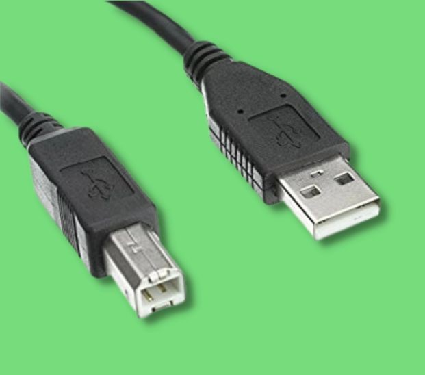
MIDI over USB cable for connecting MIDI controllers to computers.
Both cables send MIDI data. But their only difference is that USB is for computer connectivity while 5-DIN MIDI is for connecting multiple controllers together, allowing you to control them all from just one interface.
But no matter which cable is connected, both send MIDI information. And recording with MIDI isn’t the same as recording audio either way.
USB AND 5-Din cables are digital cables, meaning they transport binary/digital data.
So whether you’re pressing a key, adjusting a fader or a knob on your MIDI keyboard, these cables transport that information via digital data to your computer. But it’s not just any digital data…
That’s right, it’s sending MIDI files.
MIDI files (.MID)
MIDI files (.MID) house the digital data that we send and receive when playing with parameters on our keyboard.
.MID files do not contain any information about how a track, channel, or instrument sounds. More specifically, they only contain information about your playing of the hardware.
Whereas analog equipment relies on electrical current to transport information about parameter changes, MIDI control surfaces, keyboards, and pads rely on MIDI files for control information that determines how you’re playing on the MIDI hardware – thus affecting the sound of a virtual instrument, software synthesizer, or adjusting plugin/DAW parameters.
Then your computer reads and executes the commands in these files; playing equivalent notes or adjusting settings based on your commands.
Examples of data sent in MIDI files:
- Note duration
- Note velocity (how fast and how much pressure)
- Global controls: play, record, stop
- Pitch bend
- Modulation amount
Composing with MIDI
As we saw earlier, a MIDI recording looks very different to an audio recording. Where an audio recording gives us a waveform, a MIDI recording gives us blocks.
These blocks are MIDI notes. While they couldn’t look any more computeristic, these notes are full of the MIDI data that represents your musical technique while playing on the MIDI equipment.
When the DAW’s metronome reaches a MIDI sequence, the DAW will process this data and output the resulting sound.
MIDI keyboards vs standalone keyboards
I think this makes for a good time to highlight the difference between MIDI keyboards and standalone keyboards. That is, MIDI keyboards generally don’t have any onboard sounds of their own whereas standalone keyboards do.
And if they do, like the AKAI MPK Mini MK 3, you’ll still need accompanying software to use them.
So rather than playing a characteristic sound of the keyboard, what does play is the virtual instrument it’s controlling – including the audio result of parameters changes made while recording like pitch bend.
So MIDI keyboards do emulate standalone keyboards and pianos with some added digital functionality – I have never seen a pitch bend wheel on a piano. They are just a means of controlling sounds on your computer.
Virtual instruments
A virtual instrument is a software tool that emulates the sound of an instrument or multiple instruments.
Developers sample physical instruments with different recording techniques and in different locations to capture different characteristics of the sound too.
Then, they turn these recordings into a virtual recreation of that instrument!
If you wanted to be a musician 100 years ago you’d have needed a physical instrument. And if you didn’t have a big wallet in spare cash when the first synth entered the market you’d be hard-pressed to find one you could afford.
But thanks to digital audio we now have (much cheaper) virtual instruments and software synthesizers.
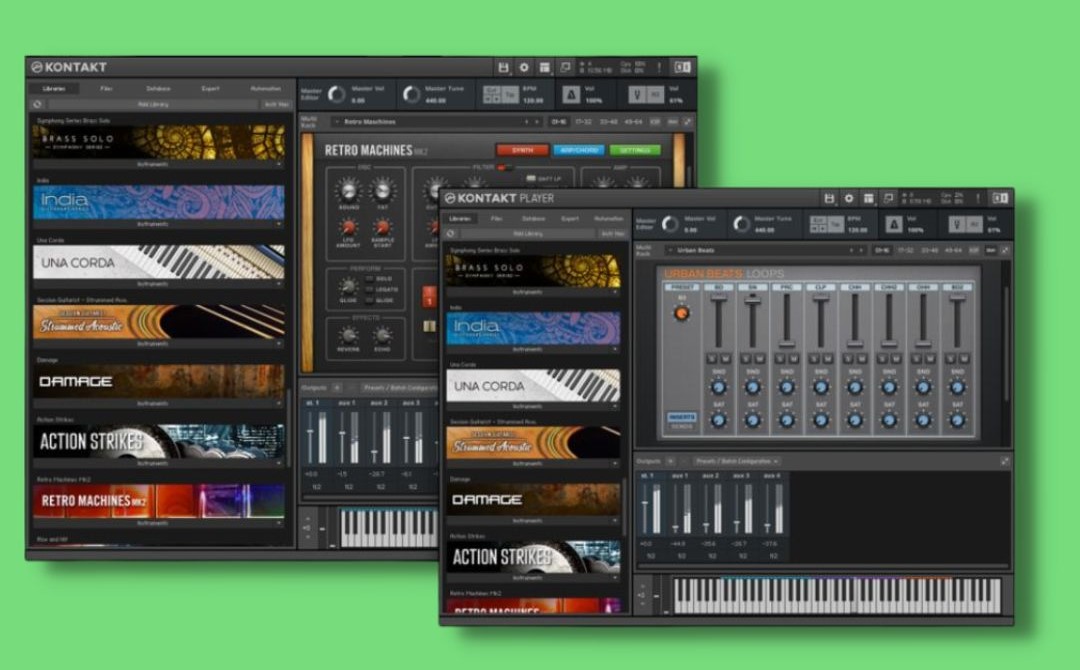
As a result, we can write music with instruments that we don’t own in the physical realm – but we do in the digital space. The most notorious virtual instrument software is Kontakt by Native Instruments.
Software synthesizers
Like a hardware synth, a software synthesizer is a program for generating your own sounds.
Soft synths are far cheaper than hardware synths – they don’t really go higher than $150!
There are a number of different types of synthesizers that use different styles of synthesis to produce sound. The most popular today is wavetable synthesis.
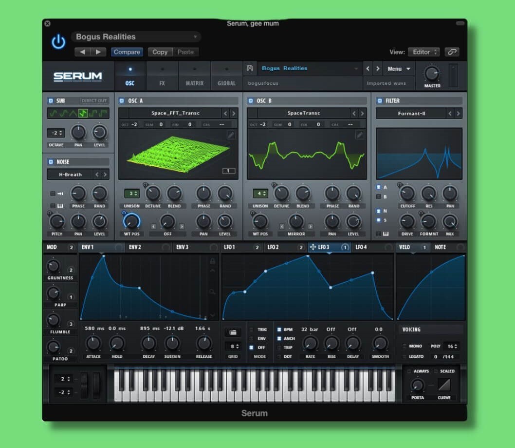
A software synthesizer utilizes the same basic principles as a hardware synthesizer, but each synth has its own characteristic tools and effects too.
Universal synthesizer features include:
- Oscillators for generating a signal
- Amplitude envelopes for shaping the sound
- Filters for refining the sound
- LFOs and additional envelopes for applying various modulations to multiple settings
When the first consumer hardware synths entered the market – like the Roland Juno – electronic music grew in popularity with speed.
Now, electronic music is a huge part of the music industry and it’s more affordable than ever to make your own sounds without breaking the bank.
FX plugins
Plugins are pieces of software that we can use to apply effects to our audio.
Before digital, all music production was hardware based with analog technology. Effects like compression and EQ would be standalone pieces of equipment (outboard gear) which were expensive and certainly not small.
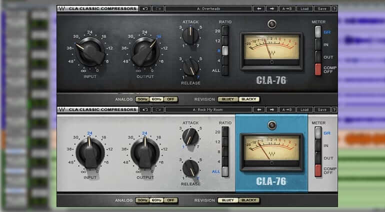
Illustrative examples are plugin emulations of expensive outboard gear. In the mid 60’s, Universal Audio’s CLA 1176 compressor rack unit was (and still is) all the rage. But it’s a pretty expensive unit.
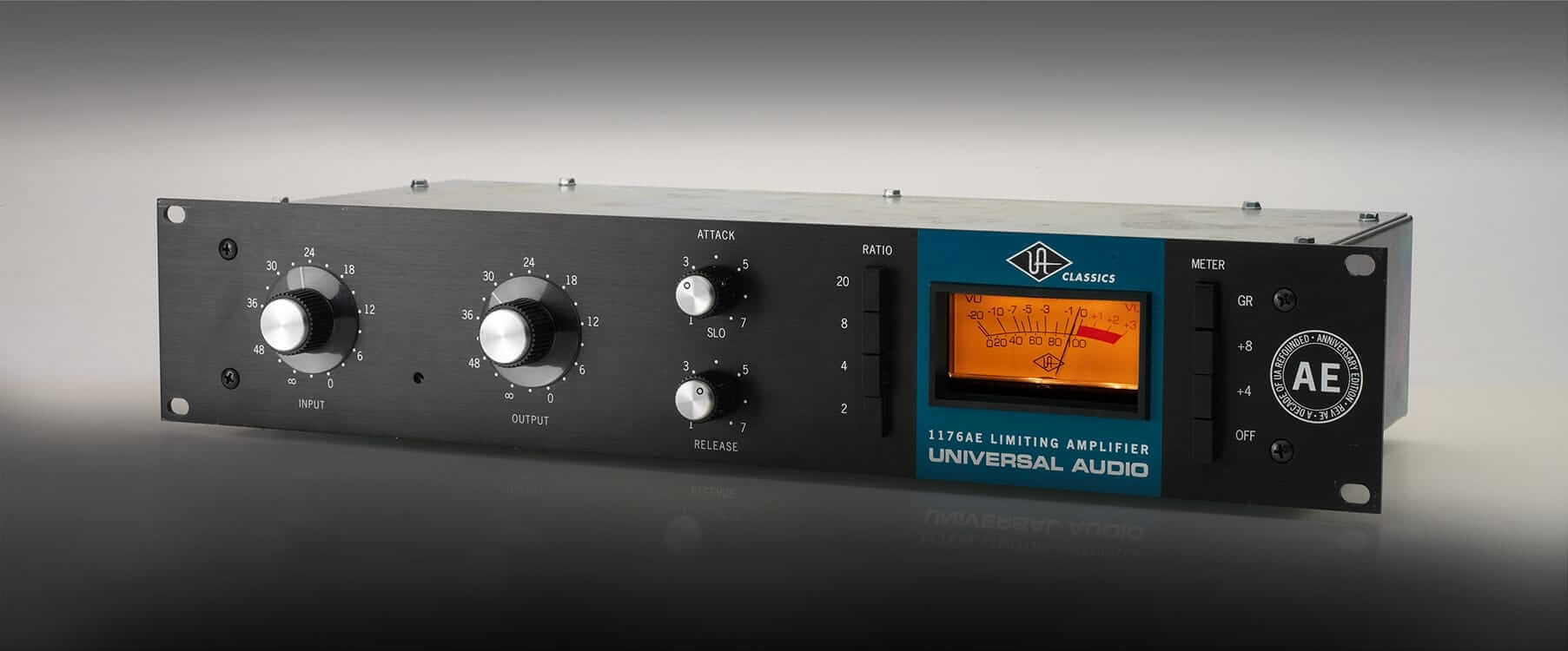
However, today you can pick up plugin emulations of the unit for a fifth of the price!
Plugins digitally emulate specific or multiple effects and reside solely on our they live on our computers. Developers build plugins to integrate with our DAWs so we can insert them on single channels or groups of channels.
Whereas today we can insert a reverb plugin onto a channel strip, recording engineers would often manually record time-based effects like reverb and delay by having artists perform in a room with lots of inherent reverb in its room signature.
The price of FX plugins can vary depending on what they offer, but they’re much more affordable than hardware units!
What is latency in digital audio recording?
Despite their differences, audio & MIDI recording have a common enemy: latency.
Latency is a time delay between your input of an instruction such as ‘Play’, striking a MIDI note, or hitting ‘Record’ your computer executing your command or registering your input. So when latency occurs with an instruction such as ‘Play’, there is a delay in time before you hear any playback.
If you’ve ever tried writing words with a slow laptop, you’ll have experience latency first-hand. The forever-seeming delay between your key press and resulting letter generation is latency!
Due to all of the calculations occurring in digital audio, latency can often disrupt your creative process. It can accumulate anywhere in your signal chain and can be as long as a few milliseconds to a few seconds.
Here are some examples:
- 0-11ms is an unnoticeable amount of latency.
- 11-22 ms delay is audible latency and it sounds like a slapback effect (think slapback delay).
- Anything more than 22 ms makes it impossible to perform in time with a track.
If you do experience latency in your digital audio setup there are a number of things you can do to solve the problem.
- Windows users can use ASIO4ALL universal low-latency drivers.
- Decrease your DAW buffer settings to the shortest time your computer can process without crashing, distorting the audio, or freezing.
- While performing, the ‘direct monitor’ feature on your audio interface allows you to hear your audio signal as you play it.
- If you’re using low-latency drivers in Windows, make sure your interface isn’t set to be a plug-and-play device.
Exporting your digital music production
Exporting your project is the final step of production. Often referred to as “bouncing” or “freezing”, exporting your audio is simply converting the DAW project into an audio file.
In addition to exporting the final master project, there are scenarios in the production process where producers export unfinished projects too!
For instance, the more processor-hungry effect plugins you insert will slow your system down as the project plays, especially those with less than 16GB of RAM.
Therefore it’s necessary to export that loop and all of its effects to a singular audio file. That way, you can reinsert the audio, play it in the context of the track, and eat up less processing power.
Additionally, it’s somewhat of a standard to “bounce” a final mixdown to a handful of audio files; known as “stems“.
And collaborating with artists across different DAWs is made possible by exporting “multitracks” rather than stems.
Multitracks
Multitracks are exports of every DAW channel of a project.
They’re the individual elements. From an individual kick sample to a 16-bar guitar loop. Furthermore, multitracks are defined by their channel name in the project. For example:
- Kick 1
- Kick 2
- Bass slide
- Guitar loop 1
- Snare
- Crash Hat 1
- Crash Hat 2
Further examples of multitracks include clap loops, drum fills, and vocal adlibs too.
Multitracks can be mono or stereo – it all depends on what the multitrack is. After all, you wouldn’t export a bass sample in stereo!
We would utilize multitrack when we’re collaborating with other musicians with different DAWs. Due to how DAWs have their own project file types, we need to export our channels to audio files if we want a collaborator to be able to do anything with them.
When our collaborator inserts the multitrack files into their DAW, the samples will jump to where they were sitting in your own DAWs timeline!
Stems
If multitrack are individual channel exports, stems are groups of channels. They’re effectively the layers of your project!
The channel groupings themselves are dictated by instrument groups and their pace in the mix. For example:
- ‘Drums’
- ‘Leads’ – lead instruments
- ‘Vocals’
- ‘Bass’
- ‘Pads’
So playing every stem together simultaneously plays your whole project as you made it. Though there aren’t really any written rules, a mastering engineer may have a preference for what should be grouped with what to get the best results.
A mastering engineer will ask for project stems rather than a whole-project export because stems offer creative control to make more precise adjustments.
Digital audio file formats
Finally, let’s talk about the digital audio file formats. Different digital file types have different characteristics and can offer you something different, and the file type best to export to depends on your needs.
You’ve heard of MP3 files, and possibly FLAC and WAV file types. These are three of the common file types, but streaming stores only accept MP3 or FLAC file types for reasons we will soon explore.
.MP3
First, let’s talk about the most popular file format.
MP3 files are a lossy file format. Lossy is one of three techniques of compressing a digital file in size for storage.
Lossy file formats such as MP3 have audio content that human ears have difficulty with hearing or can’t hear removed to reduce the size of the file. Additionally, parts of the audio that make next to no difference to the sound of the project are discarded too.
While often a subject of debate, an advantage of MP3 files is the drastic reduction in file size; making them a good choice for preserving storage space on limited-capacity devices.
But their reduced size also gives MP3s the advantage of fast distribution over the internet. And that, you guessed it, is why streaming stores like Spotify use MP3 files.
So if your project is finished and ready for the ears of your fans, export it to an MP3 and get it online!
.FLAC
FLAC files are the most popular lossless file format.
Lossless file formats don’t cut any of the audio away like lossy formats. However, they do cut the file up.
FLAC holds second place on the podium of general file type popularity – just behind MP3 files. However, because no audio is cut away in the compression process the file size can be double that of an MP3.
To illustrate how lossless compression works, let’s get hands-on.
Moving house can require fitting a king-size bed through small doors. After trying every possible angle, you’ll realize that it’s far better to disassemble the bed and transport its pieces to your new place before reassembling it.
And this is how lossless compression works! The file is snipped into smaller pieces to preserve storage space and reassembled perfectly when you load and play the file. In contrast to lossy files, lossless compression maintains sound quality and accounts for every piece of audio data.
Though they can be double the file size of MP3s and therefore slower to transport across the internet, it’s the price to pay if you’re a die-hard audiophile.
.WAV
Finally, we have WAV files. A hard drive’s worst nightmare, but an audiophile’s best friend.
WAV files are often confused as to being a lossless file type, but this isn’t true. They are a PCM file format.
PCM (Pulse Code Modulation) files actually replicate the ADC process that we have discussed at length! The difference, of course, is that we’re resampling the digital signal rather than an electrical analog signal.
PCM file types take thousands of snapshot samples of the project in question and accurately represent the original audio. As the Nyquist-Shannon theory suggests, PCM files sample each wave cycle twice to read the frequency accurately.
As a result, PCM files can be double the size of lossless file types. PCM files are the biggest storage space swallowers, but as the file isn’t compressed or cut whatsoever they have incredible audio fidelity.
And it’s for their audio fidelity that PCM file types like WAV are the industry’s favorite choice when exporting to stems and multitrack. When the time comes, export your stems/multitracks to WAV to preserve the audio quality for mixing/mastering.
Final thoughts
It was in the late 80s and early 90s that music production and recording became so accessible. 20 years later, a jaw-dropping number of artists record and release their music independently of record labels.
But 50 years ago, reel-to-reel tape decks were revolutionary tools for professional recording. But thanks to the unlimited possibilities of digital, the landscape of the music industry has changed – and continues to change – forever.
Now that you understand how digital audio works and how it empowers anyone with a computer to express themselves musically, isn’t it time you joined the millions of independent artists around the world in changing the music industry?